Getting Started

Installation

Clone the repository and install with uv:

git clone <repo-url>
cd mutation_game
uv sync

This installs all runtime dependencies (numpy, networkx, matplotlib).

Basic Usage

Create a game from a Dynkin diagram

The quickest way to get started is with a named Dynkin diagram:

from mutation_game import MutationGame

game = MutationGame.from_dynkin("A3")

Supported types: A1–An, D4–Dn, E6, E7, E8.

Create a game from an adjacency matrix

You can also supply an explicit adjacency matrix:

adj = [
    [0, 1, 0],
    [1, 0, 1],
    [0, 1, 0],
]
game = MutationGame(adj)

Performing mutations

Set an initial population and mutate individual nodes:

game = MutationGame.from_dynkin("A3")
game.set_starting_population([1, 0, 0])

print(game.mutate(0))  # [-1,  0,  0]
print(game.mutate(1))  # [-1, -1,  0]

The mutation game rule at node k is:

Invert the population of the chosen node and add the populations of all its neighbors: new[k] = -old[k] + sum(neighbors of k)

Mutation as matrix multiplication

This rule is a linear transformation. For each node k, the mutation matrix M_k is the identity matrix with row k replaced:

\[\begin{split}(M_k)_{ij} = \begin{cases} -1 & \text{if } i = k \text{ and } j = k \\ \text{adj}_{kj} & \text{if } i = k \text{ and } j \neq k \\ \delta_{ij} & \text{if } i \neq k \end{cases}\end{split}\]

Example – A3, mutation at node 1

The A3 graph is 0 — 1 — 2, with adjacency matrix:

\[\begin{split}A = \begin{pmatrix} 0 & 1 & 0 \\ 1 & 0 & 1 \\ 0 & 1 & 0 \end{pmatrix}\end{split}\]

Node 1 has neighbors 0 and 2. The mutation matrix M_1 starts as the identity, then row 1 is replaced with [adj(1,0), -1, adj(1,2)] = [1, -1, 1]:

\[\begin{split}M_1 = \begin{pmatrix} 1 & 0 & 0 \\ 1 & -1 & 1 \\ 0 & 0 & 1 \end{pmatrix}\end{split}\]

Applying it to the vector v = (3, 1, 2):

\[\begin{split}M_1 \begin{pmatrix} 3 \\ 1 \\ 2 \end{pmatrix} = \begin{pmatrix} 3 \\ 3 - 1 + 2 \\ 2 \end{pmatrix} = \begin{pmatrix} 3 \\ 4 \\ 2 \end{pmatrix}\end{split}\]

Node 1’s value changed from 1 to -1 + 3 + 2 = 4, while the other nodes are unchanged.

Applying mutation k is then simply v' = M_k @ v. You can access these matrices directly:

>>> game = MutationGame.from_dynkin("A3")
>>> print(game.mutation_matrix(1))
[[ 1  0  0]
 [ 1 -1  1]
 [ 0  0  1]]

Note that each M_k is an involution: M_k @ M_k = I. This means mutating the same node twice restores the original vector.

Computing the root system

game = MutationGame.from_dynkin("A3")
roots = game.calculate_roots()
print(f"A3 has {len(roots)} roots")  # 12

The method explores all reachable vectors by BFS over every possible mutation sequence, starting from the simple roots e_i and -e_i. It first checks that the Cartan matrix is positive definite (see Mathematical Background), ensuring the root system is finite. For non-finite-type graphs, a RuntimeError is raised immediately.

Known root counts:

Type	Total roots
A_n	n(n + 1)
D_n	2n(n - 1)
E₆	72
E₇	126
E₈	240

Finding mutation paths

Given two roots, find_mutation_path returns the shortest sequence of mutations to transform one into the other:

>>> game = MutationGame.from_dynkin("A3")
>>> path = game.find_mutation_path([1, 0, 0], [1, 1, 1])
>>> for mut_idx, result in path:
...     print(f"  mutate node {mut_idx} -> {list(map(int, result))}")
  mutate node 1 -> [1, 1, 0]
  mutate node 2 -> [1, 1, 1]

Starting from the simple root (1, 0, 0), we reach (1, 1, 1) in two mutations: first mutate node 1, then node 2.

Each step is a (mutation_index, resulting_vector) pair. The method raises ValueError if either vector is not a root in the system.

Mutation path table

To see the shortest paths between all pairs of roots at once, use print_mutation_path_table:

>>> game = MutationGame.from_dynkin("A3")
>>> game.print_mutation_path_table()
Source     Target     Mutations         Len
-------------------------------------------
(0, 0, 1)  (0, 1, 0)  1 -> 2            2
(0, 0, 1)  (0, 1, 1)  1                 1
(0, 0, 1)  (1, 0, 0)  1 -> 2 -> 0 -> 1  4
(0, 0, 1)  (1, 1, 0)  1 -> 2 -> 0       3
(0, 0, 1)  (1, 1, 1)  1 -> 0            2
(0, 1, 0)  (0, 1, 1)  2                 1
(0, 1, 0)  (1, 0, 0)  0 -> 1            2
(0, 1, 0)  (1, 1, 0)  0                 1
(0, 1, 0)  (1, 1, 1)  0 -> 2            2
(0, 1, 1)  (1, 0, 0)  2 -> 0 -> 1       3
(0, 1, 1)  (1, 1, 0)  2 -> 0            2
(0, 1, 1)  (1, 1, 1)  0                 1
(1, 0, 0)  (1, 1, 0)  1                 1
(1, 0, 0)  (1, 1, 1)  1 -> 2            2
(1, 1, 0)  (1, 1, 1)  2                 1

By default only positive roots are included. Pass positive_only=False for the full table. The programmatic version mutation_path_table() returns a list of dicts for further processing.

Note

Each mutation is an involution (applying it twice restores the original vector), so every path is reversible: to go from B back to A, apply the same mutations in reverse order. For example, if 1 -> 2 -> 0 transforms A into B, then 0 -> 2 -> 1 transforms B back into A. This is why the table lists each pair only once.

Plotting

Positive roots (default)

By default, plot_root_orbits shows only the positive roots arranged in a hierarchical layout, with simple roots at the top:

game = MutationGame.from_dynkin("A3")
fig = game.plot_root_orbits()
fig.savefig("a3_positive.png", bbox_inches="tight", dpi=150)

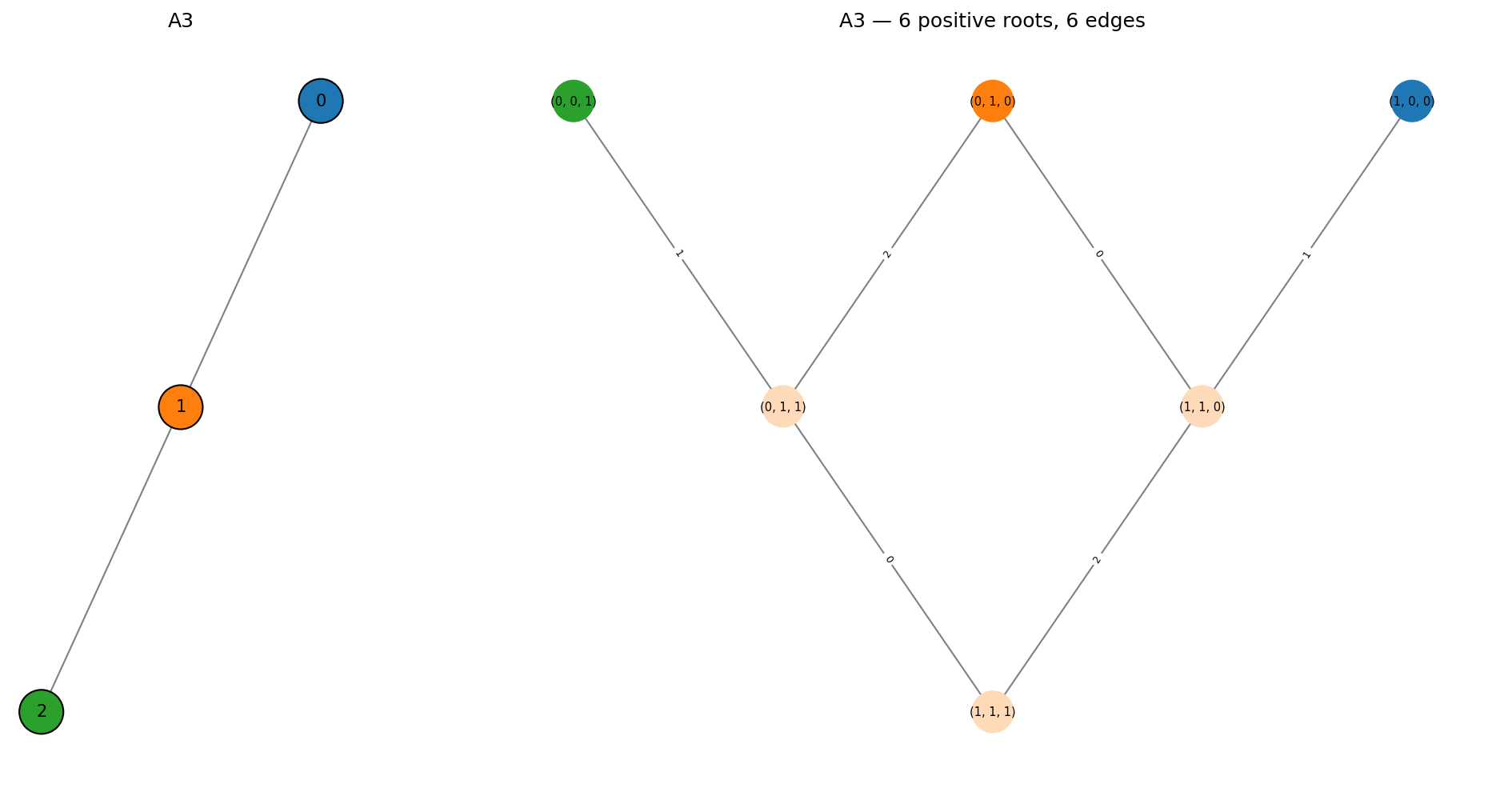
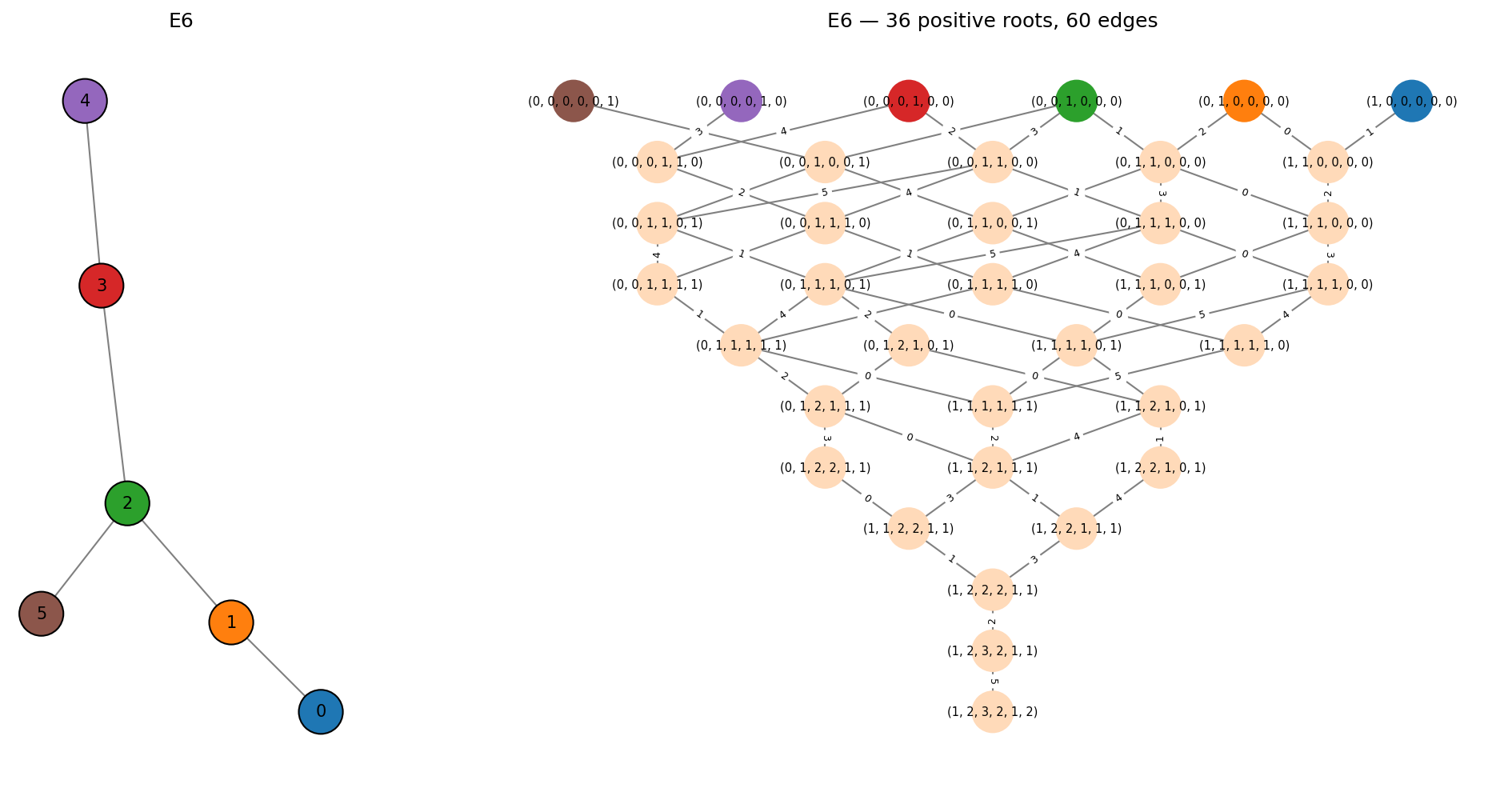
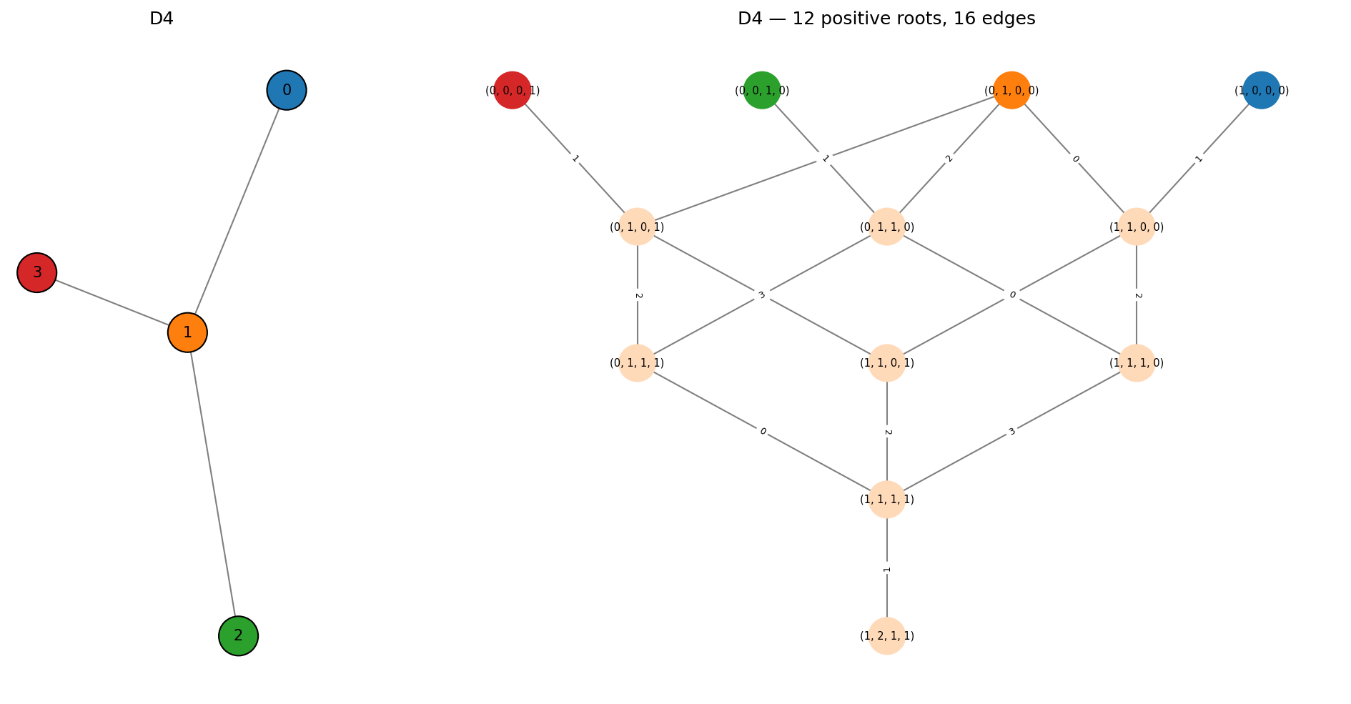
The left panel shows the input Dynkin diagram. Each node has a distinct color that matches the corresponding simple root in the mutation graph on the right. Edges in the mutation graph are labeled with the index of the mutated node.

All roots

Pass positive_only=False to see both positive and negative roots:

fig = game.plot_root_orbits(positive_only=False)
fig.savefig("a3_all.png", bbox_inches="tight", dpi=150)

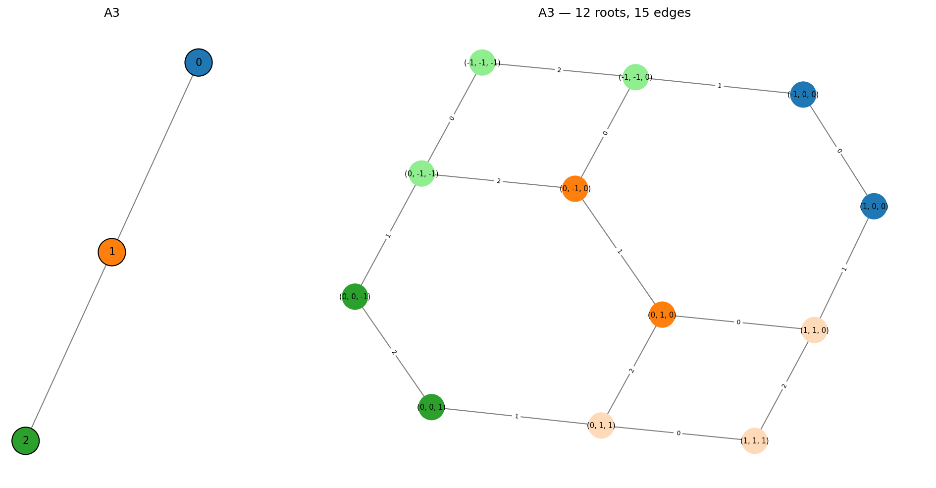
Color scheme:

Distinct color per node – simple roots +e_i and -e_i share the color of node i in the Dynkin diagram
Peachpuff – non-simple positive roots
Light green – non-simple negative roots

Larger examples

D4:

game = MutationGame.from_dynkin("D4")
fig = game.plot_root_orbits()
fig.savefig("d4_positive.png", bbox_inches="tight", dpi=150)

E6:

game = MutationGame.from_dynkin("E6")
fig = game.plot_root_orbits()
fig.savefig("e6_positive.png", bbox_inches="tight", dpi=150)