From Platonic Solids to Dynkin Diagrams

The same Diophantine inequality \(\frac{1}{p+1} + \frac{1}{q+1} + \frac{1}{r+1} > 1\) that classifies ADE Dynkin diagrams (see Proof of the ADE Classification) also classifies the Platonic solids, finite rotation groups, and spherical triangle groups. This section traces the chain of connections.

1. Euler’s Formula and Regular Polyhedra

A regular polyhedron (Platonic solid) is a convex polyhedron whose faces are congruent regular polygons and whose vertices all have the same valence. Let a regular polyhedron have:

• \(V\) vertices, each of valence \(q\) (edges meeting at each vertex)

• \(E\) edges

• \(F\) faces, each a regular \(p\)-gon

Euler’s polyhedron formula gives:

\[V - E + F = 2\]

Each edge borders 2 faces and connects 2 vertices, so:

\[pF = 2E, \qquad qV = 2E\]

Substituting into Euler’s formula:

\[\frac{2E}{q} - E + \frac{2E}{p} = 2\]

Dividing by \(2E\):

\[\frac{1}{q} + \frac{1}{p} - \frac{1}{2} = \frac{1}{E}\]

Since \(E > 0\), we need:

(1)\[\frac{1}{p} + \frac{1}{q} > \frac{1}{2}\]

with \(p \geq 3\) (faces are at least triangles) and \(q \geq 3\) (at least 3 edges meet at each vertex).

2. Enumerating Solutions

We enumerate all integer solutions of (1) with \(3 \leq p \leq q\) (by duality, swapping \(p\) and \(q\) gives the dual polyhedron):

Case \(p = 3\) (triangular faces):

\[\frac{1}{3} + \frac{1}{q} > \frac{1}{2} \quad\Longleftrightarrow\quad q < 6\]

• \(q = 3\): \(E = 6\) – Tetrahedron (4 vertices, 4 faces)

• \(q = 4\): \(E = 12\) – Octahedron (6 vertices, 8 faces)

• \(q = 5\): \(E = 30\) – Icosahedron (12 vertices, 20 faces)

Case \(p = 4\) (square faces):

• \(q = 3\): \(E = 12\) – Cube (8 vertices, 6 faces) – dual of octahedron

Case \(p = 5\) (pentagonal faces):

• \(q = 3\): \(E = 30\) – Dodecahedron (20 vertices, 12 faces) – dual of icosahedron

Case \(p \geq 6\): \(\frac{1}{p} + \frac{1}{q} \leq \frac{1}{6} + \frac{1}{6} < \frac{1}{2}\). No solutions.

That gives exactly 5 Platonic solids (3 + 2 duals). Each is labeled below with its corresponding Dynkin type – the tetrahedron corresponds to \(E_6\), the cube/octahedron dual pair to \(E_7\), and the dodecahedron/icosahedron dual pair to \(E_8\).

Interactive 3D viewer – click and drag to rotate, scroll to zoom (open fullscreen):

3. The Rotation Groups

Each Platonic solid has a rotation group – the group of orientation-preserving symmetries. Up to conjugacy, these are exactly the finite subgroups of \(SO(3)\):

Solid	\((p, q)\)	Rotation group	Order	Generators
Tetrahedron	(3, 3)	\(A_4\) (alternating)	12	3-fold and 2-fold rotations
Cube / Octahedron	(4, 3) / (3, 4)	\(S_4\) (symmetric)	24	4-fold, 3-fold, 2-fold rotations
Dodecahedron / Icosahedron	(5, 3) / (3, 5)	\(A_5\) (alternating)	60	5-fold, 3-fold, 2-fold rotations

Additionally, there are two infinite families of finite subgroups of \(SO(3)\):

• Cyclic groups \(C_n\) (rotation by \(2\pi/n\) about an axis)

• Dihedral groups \(D_n\) (rotations of a regular \(n\)-gon, including flips)

Theorem. The finite subgroups of \(SO(3)\) are exactly: cyclic \(C_n\), dihedral \(D_n\), and the three polyhedral groups \(A_4, S_4, A_5\).

4. The McKay Correspondence: From SO(3) to SU(2) to Dynkin

The rotation group \(SO(3)\) has a double cover \(SU(2)\) (the group of unit quaternions). Every finite subgroup \(G \subset SO(3)\) lifts to a binary subgroup \(\tilde{G} \subset SU(2)\) of twice the order:

\(SO(3)\) subgroup	\(SU(2)\) lift	Order	Dynkin diagram
\(C_n\) (cyclic)	Binary cyclic \(\tilde{C}_n\)	\(2n\)	\(A_{n-1}\)
\(D_n\) (dihedral)	Binary dihedral \(\tilde{D}_n\)	\(4n\)	\(D_{n+2}\)
\(A_4\) (tetrahedral)	Binary tetrahedral \(\tilde{T}\)	24	\(E_6\)
\(S_4\) (octahedral)	Binary octahedral \(\tilde{O}\)	48	\(E_7\)
\(A_5\) (icosahedral)	Binary icosahedral \(\tilde{I}\)	120	\(E_8\)

The McKay correspondence (John McKay, 1980) explains how the Dynkin diagram emerges from the group. It works as follows:

Step 1. Let \(\tilde{G} \subset SU(2)\) be a finite subgroup. The natural 2-dimensional representation \(\rho\) of \(\tilde{G}\) (inherited from \(SU(2)\)) is called the fundamental representation.

Step 2. List all irreducible representations \(\rho_0, \rho_1, \ldots, \rho_r\) of \(\tilde{G}\), where \(\rho_0\) is the trivial representation.

Step 3. For each \(\rho_i\), decompose the tensor product with the fundamental representation:

\[\rho \otimes \rho_i = \bigoplus_j a_{ij} \rho_j\]

Step 4. Build a graph with one node per irreducible representation, and \(a_{ij}\) edges between nodes \(i\) and \(j\).

Result. The graph obtained is the extended (affine) Dynkin diagram \(\tilde{A}_{n-1}\), \(\tilde{D}_{n+2}\), \(\tilde{E}_6\), \(\tilde{E}_7\), or \(\tilde{E}_8\). Removing the node corresponding to the trivial representation \(\rho_0\) gives the ordinary Dynkin diagram.

5. Spherical Triangle Groups

A spherical triangle is a triangle on the unit sphere \(S^2\) with angles \(\pi/p\), \(\pi/q\), \(\pi/r\). The triangle group \(\Delta(p, q, r)\) is generated by reflections in the sides of this triangle.

On a sphere, the angle sum of a triangle exceeds \(\pi\):

\[\frac{\pi}{p} + \frac{\pi}{q} + \frac{\pi}{r} > \pi\]

Dividing by \(\pi\):

\[\frac{1}{p} + \frac{1}{q} + \frac{1}{r} > 1\]

This is exactly the same inequality as in the ADE classification (see Proof of the ADE Classification, equation (1)), with the identification \(p \to p+1\), \(q \to q+1\), \(r \to r+1\) (the triangle group uses the actual angles, while the Dynkin classification uses arm lengths).

The spherical triangle groups are:

Triangle \((p, q, r)\)	Triangle group	Rotation subgroup	Dynkin diagram
\((2, 2, n)\)	Dihedral	\(D_n\)	\(A_{n-1}\) / \(D_{n+2}\)
\((2, 3, 3)\)	Tetrahedral	\(A_4\)	\(E_6\)
\((2, 3, 4)\)	Octahedral	\(S_4\)	\(E_7\)
\((2, 3, 5)\)	Icosahedral	\(A_5\)	\(E_8\)

When \(\frac{1}{p} + \frac{1}{q} + \frac{1}{r} = 1\), the triangle is Euclidean (flat) and tiles the plane – these correspond to the affine Dynkin diagrams. When the sum is \(< 1\), the triangle is hyperbolic.

6. The Unified Picture

All these classifications are manifestations of the same Diophantine constraint. The connections can be summarized as:

\[\frac{1}{p} + \frac{1}{q} + \frac{1}{r} > 1\]

\((p,q,r)\)	Dynkin	Platonic solid	\(SO(3)\) group	Singularity
\((2,2,n)\)	\(D_{n+2}\)	\(n\)-gon prism	Dihedral \(D_n\)	\(x^2 y + y^{n+1}\)
\((2,3,3)\)	\(E_6\)	Tetrahedron	\(A_4\)	\(x^3 + y^4\)
\((2,3,4)\)	\(E_7\)	Cube / Octahedron	\(S_4\)	\(x^3 + xy^3\)
\((2,3,5)\)	\(E_8\)	Dodecahedron / Icosahedron	\(A_5\)	\(x^3 + y^5\)

The \(A_n\) family (path graphs) corresponds to the cyclic groups and the \(x^{n+1}\) singularities. They don’t correspond to Platonic solids (which require \(p, q \geq 3\)), but rather to the simpler geometry of a regular polygon.

We can verify the Dynkin diagrams and root counts for all these types:

>>> from mutation_game import MutationGame

>>> # the five exceptional connections
>>> for name, solid in [("E6", "Tetrahedron"),
...                      ("E7", "Cube/Octahedron"),
...                      ("E8", "Dodecahedron/Icosahedron")]:
...     game = MutationGame.from_dynkin(name)
...     roots = game.calculate_roots()
...     pos = [r for r in roots if all(v >= 0 for v in r)]
...     print(f"  {name} ({solid}): {len(pos)} positive roots, {len(roots)} total")
  E6 (Tetrahedron): 36 positive roots, 72 total
  E7 (Cube/Octahedron): 63 positive roots, 126 total
  E8 (Dodecahedron/Icosahedron): 120 positive roots, 240 total

Root systems as geometric shapes

Before jumping to 3D, let us build the intuition in 2D with the simplest interesting example.

A₂: the hexagon (2D)

Where do the roots live? The \(A_2\) Dynkin diagram has 2 nodes connected by one edge: 0 — 1. The mutation game produces 6 roots: 3 positive and 3 negative. But these are just coordinate vectors in \(\mathbb{R}^2\) — abstract lists of numbers. To see the geometry, we need to understand what shape they make when drawn as points.

Step 1: Compute the roots from the mutation game.

This is the definition: the roots are whatever the mutation game produces, starting from the simple roots \((1, 0)\) and \((0, 1)\), by applying the mutation matrices \(M_0\) and \(M_1\) in every possible sequence.

>>> from mutation_game import MutationGame
>>> game = MutationGame.from_dynkin("A2")

>>> # The two mutation matrices
>>> print("M_0 ="); print(game.mutation_matrix(0))
M_0 =
[[-1  1]
 [ 0  1]]
>>> print("M_1 ="); print(game.mutation_matrix(1))
M_1 =
[[ 1  0]
 [ 1 -1]]

>>> # Start from simple root (1, 0) and apply mutations
>>> import numpy as np
>>> v = np.array([1, 0])           # simple root alpha_0
>>> print("Start:", v)
Start: [1 0]
>>> print("M_1 @ v:", game.mutation_matrix(1) @ v)   # mutate at node 1
M_1 @ v: [1 1]
>>> # (1, 1) is new! That's the third positive root.
>>> # Mutating (1, 1) at node 0:
>>> print("M_0 @ (1,1):", game.mutation_matrix(0) @ np.array([1, 1]))
M_0 @ (1,1): [0 1]
>>> # We got back to (0, 1) — the other simple root. No new roots this way.
>>> # Mutating (1, 0) at node 0 just negates it:
>>> print("M_0 @ v:", game.mutation_matrix(0) @ v)
M_0 @ v: [-1  0]
>>> # (-1, 0) is the negative of a simple root

>>> # The full BFS gives all 6 roots
>>> roots = game.calculate_roots()
>>> for r in roots:
...     print(list(map(int, r)))
[-1, -1]
[-1, 0]
[0, -1]
[0, 1]
[1, 0]
[1, 1]

So the mutation game has produced 6 roots in \(\mathbb{R}^2\): \((1,0)\), \((0,1)\), \((1,1)\), and their negatives. These are abstract vectors in the simple root basis. The question is: what shape do they make?

Step 2: Try plotting in \(\mathbb{R}^2\) directly.

These are vectors in \(\mathbb{R}^2\), so we can just plot them on a grid. Let’s do it:

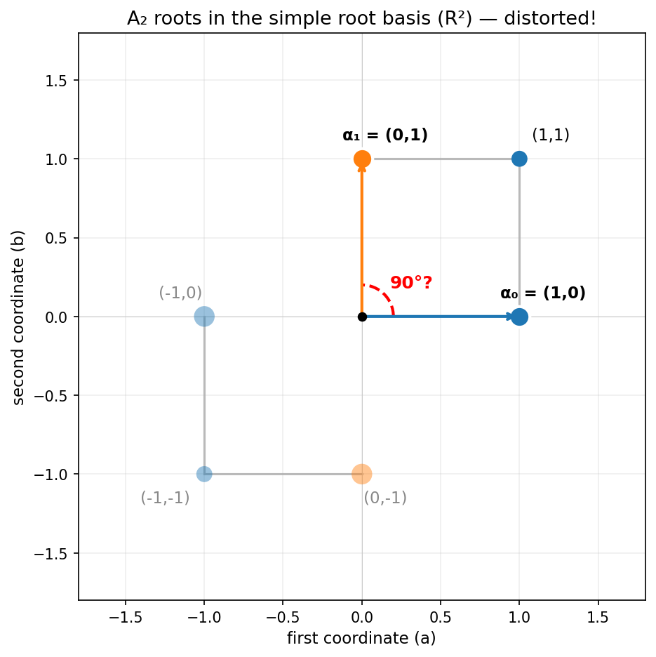
The roots form a rectangle. The two simple roots \(\alpha_0 = (1,0)\) and \(\alpha_1 = (0,1)\) appear to be at a 90-degree angle (the red dashed arc). But should we trust this picture?

When we plot points on a grid, we are implicitly using the standard dot product to measure angles and distances: \(u \cdot v = u_1 v_1 + u_2 v_2\). In the standard dot product, \((1,0)\) and \((0,1)\) are perpendicular by definition. But the root space has its own natural way of measuring angles, given by the Cartan matrix. Let’s see what it says.

The Cartan inner product. Recall from the Mathematical Background that the Cartan matrix \(C = 2I - A^T\) encodes the structure of the root system. We can use it to define an inner product — a generalization of the dot product that “knows about” the geometry of the roots.

Given two vectors \(u\) and \(v\) (expressed in the simple root basis), their Cartan inner product is:

\[\langle u, v \rangle = u^T \, C \, v\]

This looks like the dot product \(u \cdot v\), but with the matrix \(C\) inserted in the middle. When \(C\) is the identity matrix, this reduces to the ordinary dot product. When \(C\) has off-diagonal entries (as it does for \(A_2\)), it “mixes” the components, changing how angles are measured.

For \(A_2\), the Cartan matrix is \(C = \bigl(\begin{smallmatrix} 2 & -1 \\ -1 & 2 \end{smallmatrix}\bigr)\). Let’s compute the inner products of the simple roots step by step.

Length of \(\alpha_0 = (1, 0)\):

\[\begin{split}\langle \alpha_0, \alpha_0 \rangle = \begin{pmatrix} 1 & 0 \end{pmatrix} \begin{pmatrix} 2 & -1 \\ -1 & 2 \end{pmatrix} \begin{pmatrix} 1 \\ 0 \end{pmatrix} = \begin{pmatrix} 1 & 0 \end{pmatrix} \begin{pmatrix} 2 \\ -1 \end{pmatrix} = 2\end{split}\]

Length of \(\alpha_1 = (0, 1)\):

\[\begin{split}\langle \alpha_1, \alpha_1 \rangle = \begin{pmatrix} 0 & 1 \end{pmatrix} \begin{pmatrix} 2 & -1 \\ -1 & 2 \end{pmatrix} \begin{pmatrix} 0 \\ 1 \end{pmatrix} = \begin{pmatrix} 0 & 1 \end{pmatrix} \begin{pmatrix} -1 \\ 2 \end{pmatrix} = 2\end{split}\]

Both simple roots have the same length (\(\sqrt{2}\) in the Cartan metric). So far, same as the standard dot product would give.

Inner product between \(\alpha_0\) and \(\alpha_1\):

\[\begin{split}\langle \alpha_0, \alpha_1 \rangle = \begin{pmatrix} 1 & 0 \end{pmatrix} \begin{pmatrix} 2 & -1 \\ -1 & 2 \end{pmatrix} \begin{pmatrix} 0 \\ 1 \end{pmatrix} = \begin{pmatrix} 1 & 0 \end{pmatrix} \begin{pmatrix} -1 \\ 2 \end{pmatrix} = -1\end{split}\]

Here is the key difference: the standard dot product gives \((1,0) \cdot (0,1) = 0\) (perpendicular), but the Cartan inner product gives \(-1\) (not perpendicular at all).

The angle. The angle \(\theta\) between two vectors satisfies:

\[\cos\theta = \frac{\langle u, v \rangle} {\sqrt{\langle u, u \rangle \cdot \langle v, v \rangle}}\]

This is the same formula as for the ordinary dot product, but using the Cartan inner product. Plugging in:

\[\cos\theta = \frac{-1}{\sqrt{2 \cdot 2}} = -\frac{1}{2} \quad\Longrightarrow\quad \theta = 120°\]

The simple roots actually meet at 120 degrees, not 90. Our \(\mathbb{R}^2\) plot used the standard dot product to draw the grid, which assumes the basis vectors are perpendicular. Since they aren’t (under the Cartan metric), the picture is distorted.

Step 3: Finding a space where the geometry is honest.

We want to draw the roots in a way that shows the true angles and distances. That means we need to find concrete vectors in some \(\mathbb{R}^m\) (with the ordinary dot product) whose dot products match the Cartan inner products. Specifically, we need two vectors \(v_0, v_1 \in \mathbb{R}^m\) such that:

\[v_0 \cdot v_0 = 2, \qquad v_1 \cdot v_1 = 2, \qquad v_0 \cdot v_1 = -1\]

Can we do this in \(\mathbb{R}^2\)? We need two vectors of length \(\sqrt{2}\) at a 120-degree angle. Yes — for example \(v_0 = (\sqrt{2}, 0)\) and \(v_1 = (-\frac{1}{\sqrt{2}}, \frac{\sqrt{6}}{2})\). That works but looks ugly.

There is a much cleaner choice in \(\mathbb{R}^3\). Consider the differences of standard basis vectors:

\[v_0 = e_1 - e_2 = (1, -1, 0), \qquad v_1 = e_2 - e_3 = (0, 1, -1)\]

Check the dot products (ordinary dot product in \(\mathbb{R}^3\)):

\[v_0 \cdot v_0 = 1 + 1 + 0 = 2 \quad\checkmark\]

\[v_1 \cdot v_1 = 0 + 1 + 1 = 2 \quad\checkmark\]

\[v_0 \cdot v_1 = 0 + (-1) + 0 = -1 \quad\checkmark\]

All three match. So the embedding \(\alpha_0 \mapsto e_1 - e_2\), \(\alpha_1 \mapsto e_2 - e_3\) is not arbitrary — it is the unique (up to rotation) simplest embedding where the ordinary dot product reproduces the Cartan inner product. We use \(\mathbb{R}^3\) (not \(\mathbb{R}^2\) or \(\mathbb{R}^{17}\)) because 3 = n+1 is the smallest dimension where this clean construction works for \(A_n\).

Now define the standard basis of \(\mathbb{R}^3\):

\[e_1 = (1, 0, 0), \quad e_2 = (0, 1, 0), \quad e_3 = (0, 0, 1)\]

The simple roots of \(A_2\) are embedded as:

\[\alpha_0 = e_1 - e_2 = (1, -1, 0), \qquad \alpha_1 = e_2 - e_3 = (0, 1, -1)\]

These are the two vectors that correspond to the nodes of the Dynkin diagram. They are the “building blocks” that generate all the roots.

Step 4: Translate all 6 roots into \(\mathbb{R}^3\).

Each root \((a, b)\) in the simple root basis means \(a \cdot \alpha_0 + b \cdot \alpha_1\):

\[\begin{split}\begin{array}{rcccl} (1, 0) &=& 1 \cdot \alpha_0 + 0 \cdot \alpha_1 &=& e_1 - e_2 = (1, -1, 0) \\ (0, 1) &=& 0 \cdot \alpha_0 + 1 \cdot \alpha_1 &=& e_2 - e_3 = (0, 1, -1) \\ (1, 1) &=& 1 \cdot \alpha_0 + 1 \cdot \alpha_1 &=& e_1 - e_3 = (1, 0, -1) \\[6pt] (-1, 0) &=& -\alpha_0 &=& e_2 - e_1 = (-1, 1, 0) \\ (0, -1) &=& -\alpha_1 &=& e_3 - e_2 = (0, -1, 1) \\ (-1, -1) &=& -\alpha_0 - \alpha_1 &=& e_3 - e_1 = (-1, 0, 1) \end{array}\end{split}\]

Look at the result: the 6 roots in \(\mathbb{R}^3\) are exactly all differences \(e_i - e_j\) with \(i \neq j\). This is not a definition — it is a consequence of the mutation game. The mutations happened to produce precisely the vectors that can be written as \(e_i - e_j\).

Each negative root is the opposite of a positive root: \(-(e_1 - e_2) = e_2 - e_1\).

Step 5: All roots lie on a plane. Check the coordinates — every root has components that sum to zero:

\[(1) + (-1) + (0) = 0, \quad (0) + (1) + (-1) = 0, \quad \text{etc.}\]

This means all 6 vectors lie on the plane \(x + y + z = 0\) inside \(\mathbb{R}^3\). This plane passes through the origin and is 2-dimensional, so we can draw the roots as points on a flat sheet of paper.

Step 6: See the hexagon. When we project these 6 points onto the plane, they are all at the same distance from the origin (\(\sqrt{2}\)), and equally spaced at 60-degree intervals. They form a perfect regular hexagon:

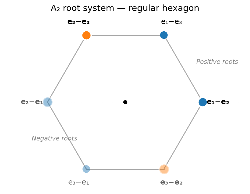
The two simple roots \(e_1 - e_2\) and \(e_2 - e_3\) (shown as larger dots with white borders) are adjacent vertices of the hexagon. The third positive root \(e_1 - e_3\) is their sum — it sits between them. The three negative roots sit on the opposite side.

Step 7: The symmetry group. The hexagon has the symmetry of an equilateral triangle (the triangle formed by the 3 positive roots). This symmetry group is \(S_3\) — the group of all permutations of 3 objects — which has \(3! = 6\) elements (3 rotations + 3 reflections).

Why \(S_3\)? Because permuting the indices \(\{1, 2, 3\}\) in \(e_i - e_j\) sends roots to roots. For example, the transposition \((1 \leftrightarrow 2)\) sends \(e_1 - e_2 \mapsto e_2 - e_1\), which swaps a positive root with its negative. This is exactly what a mutation does — and the group generated by all mutations is the Weyl group \(S_3\).

>>> # The Cartan matrix: inner products of simple roots
>>> print(game.cartan_matrix())
[[ 2 -1]
 [-1  2]]

>>> # The Coxeter element (product of both mutations)
>>> M = game.mutation_matrix(0) @ game.mutation_matrix(1)
>>> print(M)
[[ 0 -1]
 [ 1 -1]]
>>> # This matrix has order 3: M^3 = I (a 120-degree rotation of the hexagon)
>>> print(M @ M @ M)
[[1 0]
 [0 1]]

The mutation graph also forms a hexagon — the same shape! Here each node is a root vector, and the edges show which mutation transforms one root into another:

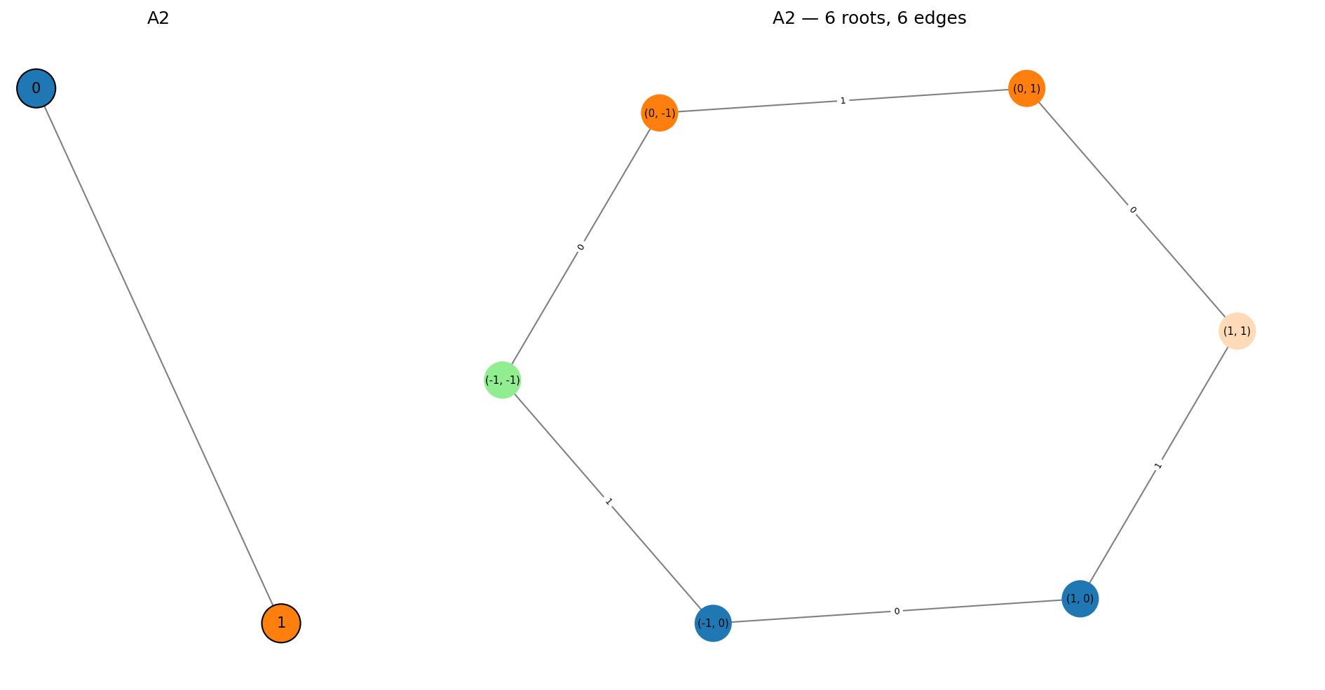
The hexagonal shape appears in both the root geometry (points in the plane) and the mutation graph (how roots are connected by mutations). This is not a coincidence — it reflects the underlying \(S_3\) symmetry.

A₃: the cuboctahedron (3D)

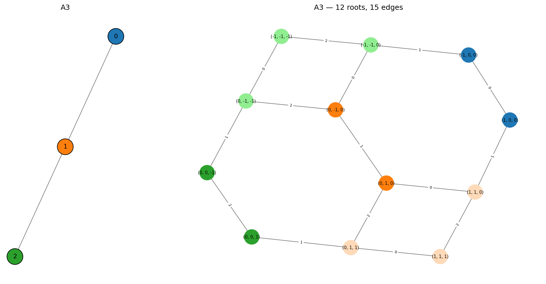
Now we go up one dimension. The \(A_3\) Dynkin diagram has 3 nodes in a path: 0 — 1 — 2. The exact same construction that gave us a hexagon in 2D now gives us a 3D shape.

Step 1: Standard basis vectors in \(\mathbb{R}^4\).

\[e_1 = (1,0,0,0), \quad e_2 = (0,1,0,0), \quad e_3 = (0,0,1,0), \quad e_4 = (0,0,0,1)\]

Step 2: Form the roots. All differences \(e_i - e_j\) with \(i \neq j\). There are \(4 \times 3 = 12\) of them — 6 positive (\(i < j\)) and 6 negative (\(i > j\)).

Step 3: Project to 3D. All 12 vectors satisfy \(x + y + z + w = 0\), so they lie on a 3-dimensional hyperplane inside \(\mathbb{R}^4\).

Step 4: See the cuboctahedron. The 12 points form a cuboctahedron — an Archimedean solid with 8 triangular faces and 6 square faces. It is the shape you get by cutting every corner of a cube at the midpoint of each edge.

Step 5: The symmetry group. The cuboctahedron has the symmetry of the cube (and its dual the octahedron). The rotation group is \(S_4\) (permutations of 4 objects, order 24) — exactly the Weyl group of \(A_3\).

The pattern:

Type	Roots	Shape	Weyl group	Symmetry of…
\(A_1\)	2	Line segment	\(S_2 = \mathbb{Z}/2\) (order 2)	—
\(A_2\)	6	Regular hexagon	\(S_3\) (order 6)	Equilateral triangle
\(A_3\)	12	Cuboctahedron	\(S_4\) (order 24)	Cube / Octahedron
\(A_4\)	20	4D polytope	\(S_5\) (order 120)	5-cell (4D simplex)

Each step up adds one dimension and one node to the Dynkin diagram, and the root polytope gains a dimension accordingly.

The mutation graph of the full \(A_3\) root system (both positive and negative roots), with 12 roots and 15 mutation edges:

The same 12 roots realized as vertices of the cuboctahedron in 3D (open fullscreen):

Each vertex of the cuboctahedron is a root \(e_i - e_j\), colored by the dominant simple root using the same tab10 palette as the mutation graph: node 0 in blue, node 1 in orange, node 2 in green. Lighter shades mark positive roots (\(i < j\)), darker shades mark negative roots. Simple roots \(e_i - e_{i+1}\) appear as larger saturated spheres.

Edges are colored by mutation index – blue edges correspond to mutation at node 0, orange to node 1, green to node 2 – matching the edge labels in the static mutation graph.

The cuboctahedral geometry reflects the \(S_4\) symmetry of the Weyl group – the same group as the rotation group of the cube/octahedron.

Note

The 240 roots of \(E_8\) can be realized as vectors in \(\mathbb{R}^8\). Their convex hull is the Gosset polytope \(4_{21}\), a remarkable 8-dimensional object with 240 vertices, 6720 edges, and deep connections to string theory and the octonions.

7. The du Val Singularities

The circle closes with the du Val singularities (also called rational double points or Kleinian singularities). Given a finite subgroup \(\tilde{G} \subset SU(2)\), consider its action on \(\mathbb{C}^2\). The quotient \(\mathbb{C}^2 / \tilde{G}\) is a surface with an isolated singularity at the origin, and this singularity is of ADE type:

Group \(\tilde{G}\)	Quotient singularity	Equation in \(\mathbb{C}^3\)	Type
Binary cyclic \(\tilde{C}_n\)	\(\mathbb{C}^2 / \tilde{C}_n\)	\(x^2 + y^2 + z^n = 0\)	\(A_{n-1}\)
Binary dihedral \(\tilde{D}_n\)	\(\mathbb{C}^2 / \tilde{D}_n\)	\(x^2 + y^2 z + z^{n-1} = 0\)	\(D_{n+2}\)
Binary tetrahedral \(\tilde{T}\)	\(\mathbb{C}^2 / \tilde{T}\)	\(x^2 + y^3 + z^4 = 0\)	\(E_6\)
Binary octahedral \(\tilde{O}\)	\(\mathbb{C}^2 / \tilde{O}\)	\(x^2 + y^3 + yz^3 = 0\)	\(E_7\)
Binary icosahedral \(\tilde{I}\)	\(\mathbb{C}^2 / \tilde{I}\)	\(x^2 + y^3 + z^5 = 0\)	\(E_8\)

The equations in the right column are exactly the ADE singularities from Arnold’s classification (see From Singularities to Dynkin Diagrams). The resolution of these surface singularities produces a configuration of exceptional curves whose intersection graph is the corresponding Dynkin diagram.

This completes the circle:

\[\boxed{\text{Platonic solid}} \to \boxed{\text{Rotation group}} \to \boxed{\text{Binary group } \tilde{G} \subset SU(2)} \to \boxed{\mathbb{C}^2 / \tilde{G}} \to \boxed{\text{ADE singularity}} \to \boxed{\text{Dynkin diagram}}\]

References

[McKay1980]

J. McKay, “Graphs, singularities, and finite groups,” Proceedings of Symposia in Pure Mathematics 37 (1980), 183–186.

[Klein1884]

F. Klein, Vorlesungen uber das Ikosaeder und die Auflosung der Gleichungen vom funften Grade, Teubner, 1884. English translation: Lectures on the Icosahedron, Dover, 2003.

[duVal1934]

P. du Val, “On isolated singularities of surfaces which do not affect the conditions of adjunction,” Proceedings of the Cambridge Philosophical Society 30 (1934), 453–459.